In the previous post about Frink, we explored how smoothly Frink handles units of measure. In this post, we will focus on another deeply integrated feature of Frink’s: interval arithmetic. On Frink’s homepage this feature is described as magical. The aim of this post is to try and make sense of this statement. We will now give a quick rundown of interval arithmetic and then proceed to concrete examples. For a more detailed review of the subject, you can refer to Wikipedia, or for a Frink-specific treatment, to the interval arithmetic section in Frink’s documentation. On with it.

Interval arithmetic 101

In interval arithmetic, instead of using numbers, we use intervals. Specifically, we say that [3, 5] represents the set of numbers between 3 and 5. Given some intervals, we can define the basic arithmetic operations on them:

1
2
3
4

[a, b] + [c, d] = [a + c, b + d]
[a, b] - [c, d] = [a - d, b - c]
[a, b] * [c, d] = [min(ac, ad, bc, bd), max(ac, ad, bc, bd)]
[a, b] / [c, d] = [min(a/c, a/d, b/c, b/d), max(a/c, a/d, b/c, b/d)]

Which should make intuitive sense if you squint hard enough. With (quite) a bit more thought, it is possible to define interval operations for more complicated functions, e.g. trigonometric functions. And that’s exactly what Frink does; most of its mathematical functions transparently support (real) intervals, so one can write:

1
2
3
4
5
6
7
8
9
10

x = new interval[-1, 4]
y = new interval[6, 9]

x + y  // => [5, 13]
x - y  // => [-10, -2]
x * y  // => [-9, 36]
x / y  // => [-1/6 (approx. -0.16666666666666667), 2/3 (approx. 0.66666666666666667)]

x^2    // => [0, 16]
sin[x] // => [-0.8414709848079, 1]

(Note that Frink uses square brackets for function application/definition.)

Although the interval definition syntax is a bit verbose and likely to change later on, the usage is indeed transparent. That is, code written for regular values (like the code above) works with intervals without any modification. Also, as can be seen in the x^2 and sin examples, applying a function to an interval is not as simple as applying the function to the interval’s boundaries, but rather involves an actual analysis of the function’s behavior on the given interval.

And that’s all we’ll need for the purposes of this post. With this rudimentary knowledge of interval arithmetic, we are now ready to try and flesh out the claim that interval arithmetic is magical.

Interval hat-trick

Suppose I want to prepare a classic hat-trick: pull a rabbit out of a top hat. For this, I would obviously need both a top hat and a rabbit. The question is, how do I make sure that the hat fits the rabbit? I can’t just order any hat, it has to be large enough to contain the rabbit.

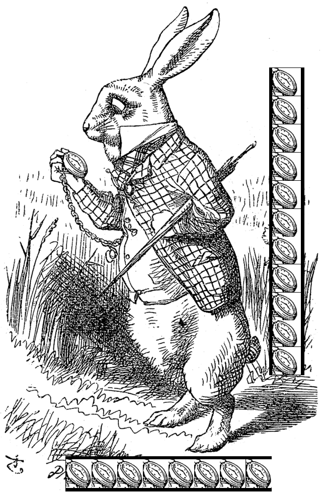
Since I know literally nothing about rabbits and their sizes, I will use the picture on the right, depicting a fairly typical rabbit, as a reference.

From this picture, we need to extract an estimate of the rabbit’s size. Luckily, the rabbit holds, as they usually do, a pocket watch, and using the handy table from this site we have an estimate of the diameter of a typical pocket watch:

1
2

pocketWatch = new interval[1.0, 1.9] inch 
// [0.0254, 0.04826] m (length)

As you can see, intervals are integrated with units; we could also have written new interval[1.0 inch, 1.9 inch], but this way is more concise.

Knowing the diameter of a pocket watch, we can draw a little “pocket watch scale” for the rabbit (on the same picture on the right). We are assuming that both the legs and the ears are foldable, so the measurement excludes this area. Looking at the picture, we can see that the rabbit is about 10.5 watches tall, and about 5 watches wide. Since I don’t really know how squishy a real rabbit is, let’s give both dimensions a bit of an error margin either way, so:

1
2

heightInWatches = new interval[10.5 - 1, 10.5 + 1]
widthInWatches = new interval[5 - 0.5, 5 + 0.5]

Combining with the size of a watch we have:

1
2
3
4
5

rabbitHeight = heightInWatches pocketWatch
// [0.2413, 0.55499] m (length)

rabbitWidth = widthInWatches pocketWatch
// [0.1143, 0.26543] m (length)

According to Wikipedia, a rabbit’s weight is:

1

rabbitWeight = new interval[0.4, 2] kg

Which means, assuming that a rabbit forms a perfect cylinder, that we can calculate the rabbit’s mass density:

1
2
3
4
5

rabbitVolume = pi (rabbitWidth / 2)^2 * rabbitHeight
rabbitDensity = rabbitWeight / rabbitVolume

rabbitDensity -> "water"
// [0.013025216116065158404, 0.8077748579515481546] water

So rabbits float on water; definitely a useful thing to know next time you go out with your rabbit to the beach. (Also, by nothing but a total coincidence, the height that we estimated fits pretty well with the data given in Wikipedia.)

Under the same cylindrical rabbit assumption, the width of the rabbit can be taken as the width of the top hat we’ll be using. From which we gather that a magician’s head circumference should be:

1
2
3
4

magicianHead = pi rabbitWidth

magicianHead -> "cm"
// [35.90840403053133671, 83.387293804233881917] cm

Which according to the table here makes the potential magician either a giant or an extraordinarily small infant.

Having done this exhaustive research, we are now ready to order a hat. Just need to figure out where one buys a top hat these days…

Okay, so what do we have here? Essentially, we just did a calculation with built-in error propagation; which in itself is quite nice (and probably useful), but as every poor-soul-of-an-undergraduate-physics-student-stuck-in-a-lab knows, error analysis is not that difficult, even without the support of special programming tools (although I’m sure that said student would show nothing but great appreciation for such a tool). So apart from the magical theme, we are yet to achieve any real magic here.

But we won’t be giving up just yet.

Interval plotting

One good use of interval arithmetic techniques is for plotting. An illustration of this can be found on a demonstration page, which generates ASCII plots for equations. As can be seen in the Frink source for this page, the code that achieves this uses interval arithmetic and is quite compact.

Let’s try to figure out how it works. Before we do that, we need something to compare to the interval arithmetic approach. Since Frink doesn’t (yet) have any built-in plotting facilities, we will roll our own simplistic plotting solution. For this purpose, we can leverage Frink’s graphics support (which is much more interesting than what I’ll be showing here, see the documentation for the full story).

Without further ado, the naive plotting solution:

1
2
3
4
5
6
7
8
9
10
11
12
13
14
15
16
17
18
19

naivePlot[lhs, rhs, xMin, xMax, yMin, yMax, xSteps, ySteps] :=
{
  g = new graphics
  g.drawRectSides[xMin, -yMin, xMax, -yMax] // a frame for the plot
  
  xStep = (xMax - xMin) / xSteps
  yStep = (yMax - yMin) / ySteps
  
  tolerance = 0.05

  multifor [x, y] = [xMin to xMax step xStep, yMin to yMax step yStep]
  {
      res = abs[lhs[x, y] - rhs[x, y]]
      if res < tolerance
        g.fillRectSize[x, -y, xStep, -yStep]
  }
  
  g.show[]
}

(the full source code for this and further snippets can be found in the repository)

The code should be fairly readable even without much familiarity with Frink. We are defining a function (as denoted by :=). The function takes two function arguments, lhs and rhs, each representing a side of the equation we are about to plot, and a bunch of numbers for the x/y limits and steps. Note that the curly braces must be on a separate line; which, from my point of view, is the only truly evil feature of Frink I’ve seen so far.

On line 3, we are initializing a new graphics object; this is the container for our plot. As a first step, on line 4, we are drawing a frame for the plot (otherwise, Frink might clip empty regions around it). Relative to standard mathematical plotting, the graphics object’s y axis is inverted, hence the minus signs on all y values.

Next, we need to step through the range of the plot; instead of using two nested loops, we are using a multifor, which combines multiple nested loops into a single construct. At every step, we are applying the lhs and rhs functions to the current x/y values and see whether they are close enough. If they are within the tolerance value, on line 15 we are drawing a filled rectangle to mark that position.

After exiting the loop, on line 18, we invoke the show method on the graphics object, which shows the result on the screen.

This is probably the crappiest plotting solution one could possibly write. The tolerance is abysmal, but since we are using a constant step, a smaller tolerance would take too many steps to achieve anything. As it is, even moderately spiky functions should throw the whole thing off. Nonetheless, this can actually plot something, and it’s good enough for illustration purposes.

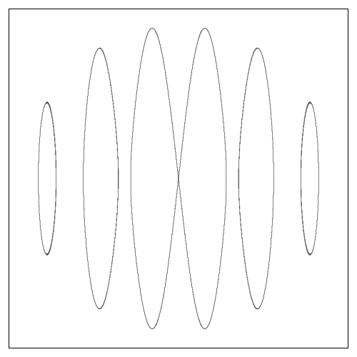
Let’s put it to the test. The preloaded example on the demonstration page plots the equation

1

x^2 + y^2 = 81 sin[x]^2

Which should result in a bunch of circles. Let’s try to apply naivePlot to draw them. First, we’ll define a pair of anonymous functions for the parts of the equation:

1
2

lhs = { |x, y| x^2 + y^2 }
rhs = { |x, y| 81 sin[x]^2 }

The { |x, y| ... } syntax defines an anonymous function with two arguments. After setting the bounds and number of steps, we can create the plot:

1
2
3
4
5
6
7
8
9
10

xMin = -10
xMax = 10

yMin = -10
yMax = 10

xSteps = 300
ySteps = 300

naivePlot[lhs, rhs, xMin, xMax, yMin, yMax, xSteps, ySteps]

And the result:

Which is reminiscent of the circles pattern we should be getting, but not quite there. We can push up the number of steps:

1

naivePlot[lhs, rhs, xMin, xMax, yMin, yMax, 800, 800]

To obtain:

Since the step size is getting smaller, the points we are drawing are tiny. But the circles are definitely visible.

Now we can proceed to the interval arithmetic variant. Here’s the code:

1
2
3
4
5
6
7
8
9
10
11
12
13
14
15
16
17
18
19

intervalPlot[lhs, rhs, xMin, xMax, yMin, yMax, xSteps, ySteps] :=
{
  g = new graphics
  g.drawRectSides[xMin, -yMin, xMax, -yMax] // a frame for the plot
  
  xStep = (xMax - xMin) / xSteps
  yStep = (yMax - yMin) / ySteps

  multifor [xx, yy] = [xMin to xMax step xStep, yMin to yMax step yStep]
  {
      x = new interval[xx, xx + xStep]
      y = new interval[yy, yy + yStep]
      
      if lhs[x, y] PEQ rhs[x, y] // doing interval comparison
        g.fillRectSize[xx, -yy, xStep, -yStep]
  }
  
  g.show[]
}

The structure of intervalPlot is quite similar to naivePlot. The key difference is that instead of applying lhs and rhs to numbers, we are applying them to intervals. Specifically, at each iteration, we are creating intervals corresponding to the numbers between the current x/y values and the next (lines 11-12). As mentioned above, Frink’s support for intervals is transparent, so we can apply lhs and rhs to the intervals in the very same way as we did in naivePlot. But now, instead of using a tolerance value to compare the results, we are using the operator PEQ, which stands for “Possibly EQuals”, i.e. it tests whether the compared intervals have some overlap. This is one of a number interval-specific operators defined in Frink (for the full list see the documentation).

In the context of plotting, PEQ is exactly what we need; given that interval arithmetic produces the right bounds, there is no way for our code to miss solutions to the equation. To make this point more clear, we can consider two single-variable functions, f and g (which for simplicity we assume to be continuous). In the previous section, it was natural to view intervals as values with an uncertainty or a measurement error. But there is another way to look at them: an interval simultaneously represents all values in its range. With this interpretation, the expression f([3, 5]) is equivalent to sampling the function on the whole range of [3, 5]. That is, the interval f([3, 5]) contains all values that f can take on the range [3, 5]. So the assertion that f([3, 5]) PEQ g([3, 5]) == false means that nowhere in the interval [3, 5] the functions f and g can be equal. That is, PEQ guarantees us that there is no solution to the equation f = g in this interval. The converse statement, f([3, 5]) PEQ g([3, 5]) == true, is not as strong, it only tells us that [3, 5] may contain a solution to the equation, but it is not guaranteed (thanks to Alan Eliasen for clarifying this point). In the code above we assume that the solution does indeed exist, and we mark it on the plot (which may yield false positives if the resulting intervals are not tight enough; though that’s beyond the scope of this post). In this way, we can achieve (paraphrasing the comment here) a “step-perfect” plot – if a solution to the equation exists within a step, PEQ cannot miss it, which contrasts probabilistic sampling methods, like naivePlot, that can miss possible solutions. Since in intervalPlot we are covering the whole plot range with intervals, we should see all solutions to the equation within the range.

Okay, but that’s all just theory, what we really need is proof, and what can better serve as a proof than a picture. For the code

1

intervalPlot[lhs, rhs, xMin, xMax, yMin, yMax, 300, 300]

we get:

Which is a bit crude, since we are not making that many steps. We should remember though, that for the equivalent step size in the naive approach, we got almost nothing at all. Here, as promised, we are not missing any solutions in the whole range. It is possible to refine the plot by increasing the step size:

1

intervalPlot[lhs, rhs, xMin, xMax, yMin, yMax, 800, 800]

and yield:

Which is quite amazing, since this solution is as simple to implement as the naive solution, but it doesn’t require us to muck about with tolerance values and step sizes, the burden of heavy lifting is on the implementation of interval arithmetic.

All this power at my fingertips… Let’s try to plot something more ambitious. For this, we’ll define the following functions:

1
2
3
4
5
6
7
8
9
10
11
12
13
14
15
16
17
18
19
20
21
22

/* A Gaussian function in one dimension */
gaussian[a, x] := exp[-x^2 / a^2]

/* A 2d Gaussian centered at (x0, y0) */
gaussian2d[a, x, x0, y, y0] := gaussian[a, x - x0] gaussian[a, y - y0]

/* A sum of 2d Gaussians with peaks at different locations. 
 * `peaks` is a list of pairs designating the positions of the peaks. 
 */
gaussians[a, x, y, peaks] :=
{
  res = 0
  for [x0, y0] = peaks
  {
     res = res + gaussian2d[a, x, x0, y, y0]
  }

  return res
}

/* A 2d surface with bumps at integer locations. */
bumps[x, y] := cos[2 pi x] cos[2 pi y]

Which is just a bunch of different bumpy functions. The sides of the equation that we will be plotting now are:

1
2

lhs = { |x, y| bumps[x, y] }
rhs = { |x, y| 2 - gaussians[0.01, x, y, peaks[]] }

Where peaks[] is a list of pairs:

1
2
3
4
5

peaks[] := [[1, 1], [1, 2], [1, 3], [1, 4], [1, 5], [2, 4], [3, 3], [4, 4], [5, 1], [5, 2], [5, 3], [5, 4], [5, 5], 
            [7, 1], [7, 2], [7, 3], [7, 4], [7, 5], [8, 3], [8, 5], [9, 3], [9, 5], [10, 1], [10, 2], [10, 3], [10, 4], [10, 5], 
            [12, 1], [12, 2], [12, 3], [12, 4], [12, 5], [13, 1], [13, 5], [14, 1], [14, 3], [14, 5], [15, 1], [15, 2], [15, 3], [15, 5], 
            [17, 1], [17, 2], [17, 3], [17, 4], [17, 5],
            [19, 1], [19, 2], [19, 3], [19, 4], [19, 5], [20, 1], [20, 5], [21, 1], [21, 5]]

The exact details of the various functions are not that important, what’s important is that both lhs and rhs can be evaluated on intervals, and so can be plotted by intervalPlot. But first, let’s see what naivePlot can make of it:

1
2
3
4
5
6
7
8
9
10

xMin = 0
xMax = 23

yMin = 0
yMax = 6

xSteps = 50
ySteps = 50

naivePlot[lhs, rhs, xMin, xMax, yMin, yMax, xSteps, ySteps]

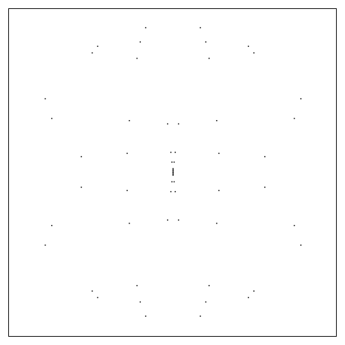
Since this function takes longer to evaluate, I won’t bother with a larger step. And the result:

One would’ve thought that with all the fuss defining the functions above, we’d have something more interesting as a result, oh well…

Let’s try intervalPlot with the same step:

1

intervalPlot[lhs, rhs, xMin, xMax, yMin, yMax, xSteps, ySteps]

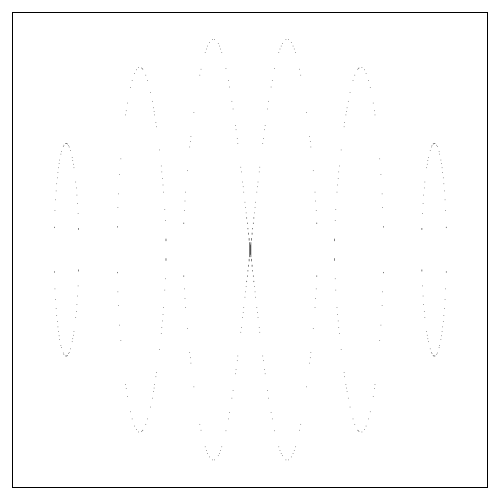
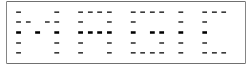
Now that’s magic!

Okay, okay, I know, it’s a bit gimmicky. Also, you might be thinking that defining some pathological function and then comparing the performance of the interval arithmetic solution to the joke of a plotting function that I came up with doesn’t really prove anything. And you’d be right, it is a somewhat inadequate comparison (though I would like to point out again how ridiculously simple intervalPlot’s implementation is). If only I had something more solid to compare to.

I’m sure that most would agree that WolframAlpha knows a thing or two about plotting. Let’s see how it compares to intervalPlot. Though it would be a bit tedious to submit our complete functions to WolframAlpha, so we’ll simplify a bit:

1
2
3
4
5
6
7
8
9
10
11

lhs = { |x, y| bumps[x, y] }
rhs = { |x, y| 2 - gaussian2d[0.01, x, 1, y, 1] }

xMin = 0
xMax = 2

yMin = 0
yMax = 2

xSteps = 50
ySteps = 50

Which is essentially the same as before, except that on line 2 we’re not using peaks[] anymore, but just a single peak. We can run

1

intervalPlot[lhs, rhs, xMin, xMax, yMin, yMax, xSteps, ySteps]

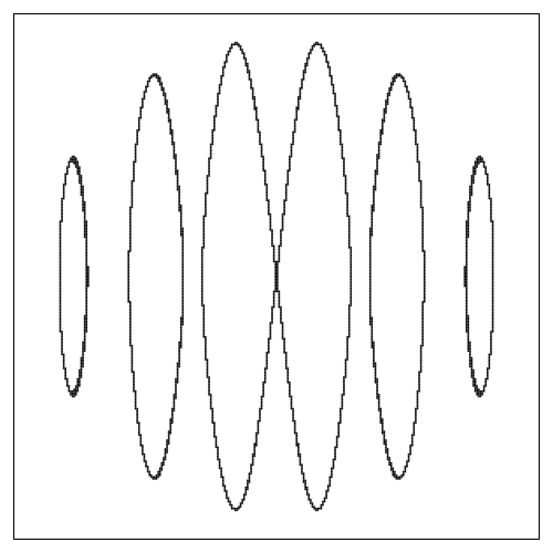
and get:

As of writing, running the equivalent expression on WolframAlpha yields the following:

Although I’ve no idea how Mathematica (and by extension WolframAlpha) implements plotting for this sort of thing, I’m sure that it’s not anywhere nearly as simple as our toy interval arithmetic function.

(Ironically, for the data above, naivePlot actually produces a plot with a point in the middle; but that’s not really a meaningful result, but rather a coincidence, since even a minor tweak, e.g. xSteps = 51, makes the point disappear. intervalPlot, is, obviously, insensitive to such tweaks.)

Having said all that, I’m not actually knowledgeable enough to be actively recommending interval arithmetic plotting solutions as a drop-in replacements for anything else. As in any other non-trivial numerical problem, I’m sure that this area has its own set of nuances, which were not apparent in the examples used in this post. Probably, the best approach to plotting is some combination of various techniques. But still, I find it quite intriguing that we managed to get so far with such a small investment.